Performance & Scaling

This page documents the performance characteristics of spark-bestfit, including scaling behavior, memory footprint, and tuning recommendations.

Note

Benchmarks were run on a local development machine. Absolute times will vary based on your hardware and cluster configuration. The key insight is the scaling characteristics: sub-linear for data size, O(D) for distribution count. Run make benchmark to generate results for your environment.

Architecture Overview

spark-bestfit uses a histogram-based approach that provides significant performance advantages over naive distribution fitting:

1. Compute histogram once: A single distributed aggregation computes the data histogram

2. Broadcast small data: Only the histogram (~8KB) and a data sample are broadcast

3. Parallel fitting: Distributions are fitted in parallel across workers

4. No data collection: Raw data never leaves the workers

This design means fit time scales sub-linearly with data size - the histogram computation is O(N) but very fast, while distribution fitting is O(1).

Time Complexity

Operation	Complexity	Notes
Data count/sample	O(N)	Single aggregation (shared across columns)
Histogram computation	O(N * C)	One histogram per column
Distribution fitting	O(C * D * B)	D distributions * B bins * C columns
Total fit time	O(N) + O(C * D * B)	Data overhead shared, fitting scales with columns

Where:

• N = number of data rows

• C = number of columns being fitted

• D = number of distributions (~90 continuous by default)

• B = histogram bins (default: 100)

Memory Footprint

Driver Memory

The driver collects minimal data:

Component	Size	Scaling
Histogram	~8 KB	O(bins) - constant
Results DataFrame	~50 KB	O(distributions)
Best results	~1 KB	O(n) for best(n=…)

Total driver overhead: < 100 KB regardless of data size.

Executor Memory

Each executor receives broadcast variables:

Component	Size	Scaling
Histogram broadcast	~8 KB	O(bins)
Data sample broadcast	~80 KB	O(max_samples) default 10K
Fitting workspace	~1 MB	Per-task temporary

Total executor overhead: < 2 MB per task - safe for most cluster configurations.

Scaling Characteristics

Data Size Scaling

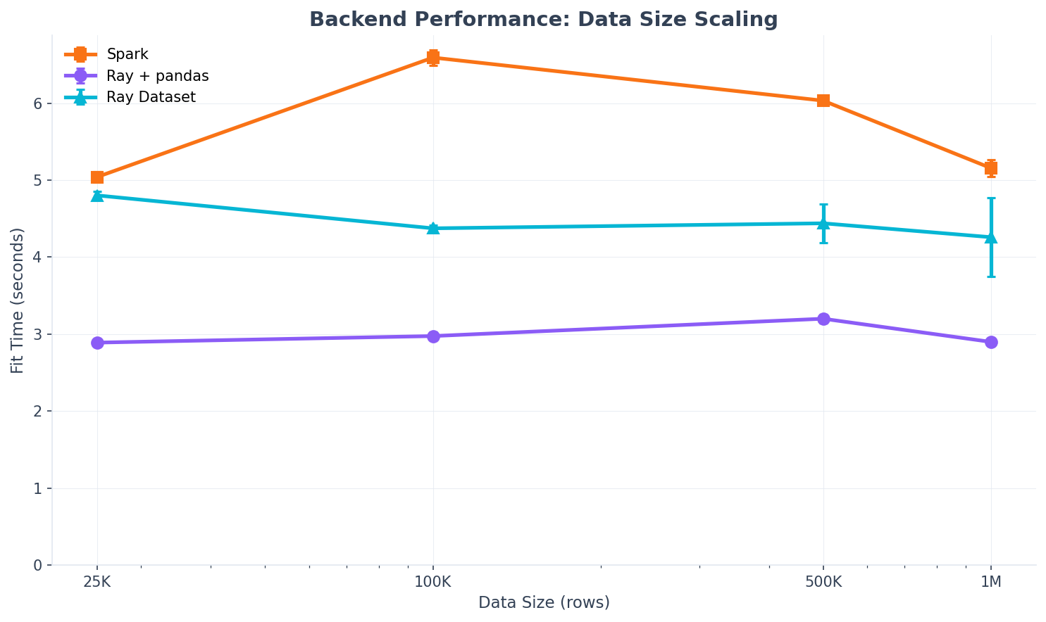
Fit time is sub-linear with data size due to the histogram-based approach. A 40x increase in data results in only ~1.0x increase in time (vs 40x if O(N)).

Note

Why times appear nearly flat: The histogram-based architecture means actual fitting operates on a fixed-size working set (~100 bins, ~10K samples), not raw data. The dominant cost is fitting ~90 distributions, which takes 2-5 seconds regardless of input data size.

Distribution Count Scaling

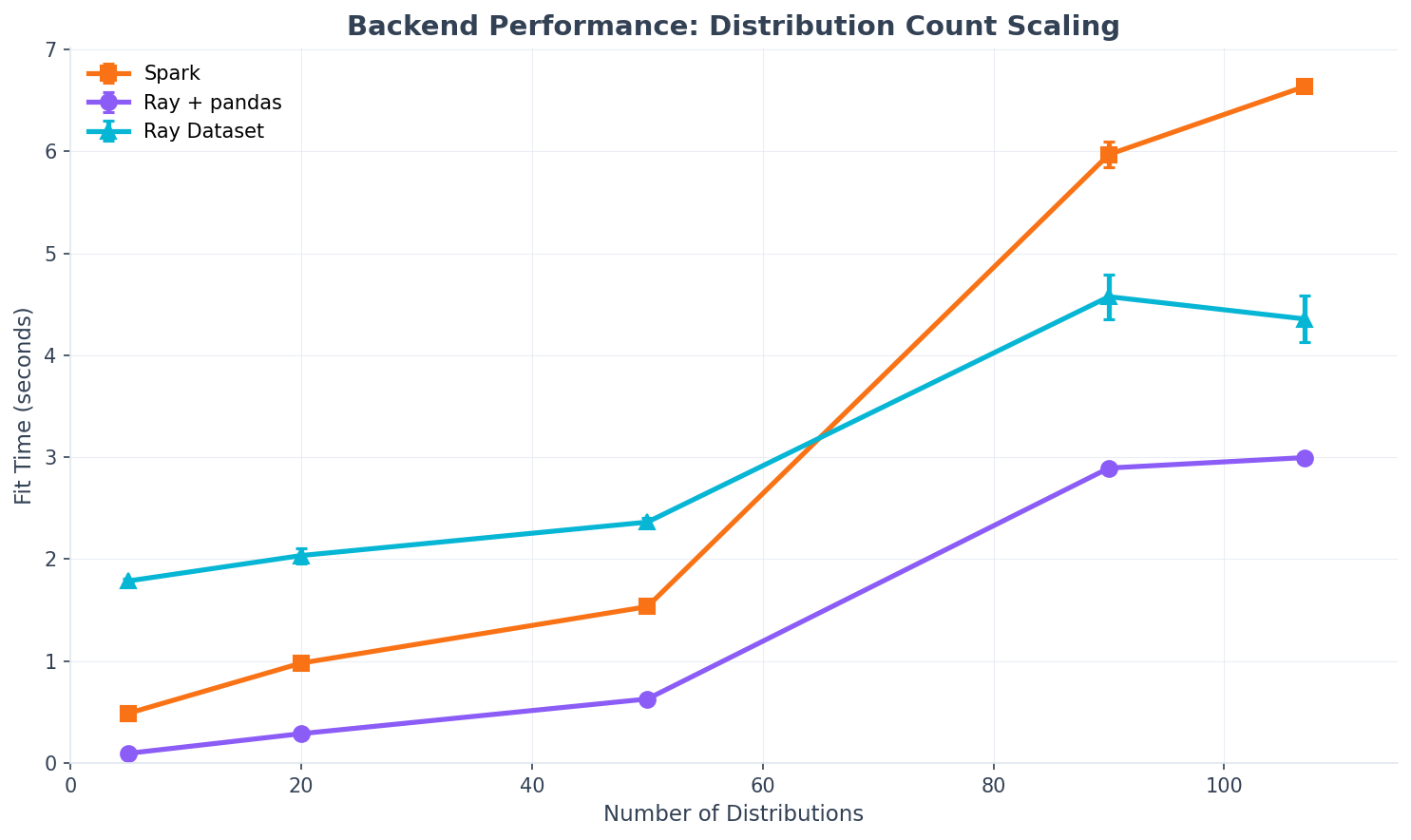
Fit time scales with the number of distributions, but not uniformly - some scipy distributions are computationally expensive:

# Distributions	Fit Time	Notes
5	~0.5s	Fast distributions only
50	~1.5s	Mix of fast/medium
90 (default)	~5-6s	Includes slow distributions

The first ~50 distributions are fast (~30ms each). The remaining distributions include slower ones like burr, t, and johnsonsb (~100-160ms each).

Spark Configuration

For optimal performance, configure your SparkSession:

from pyspark.sql import SparkSession

spark = (
    SparkSession.builder
    .appName("DistributionFitting")
    # Enable Arrow for efficient serialization
    .config("spark.sql.execution.arrow.pyspark.enabled", "true")
    # Enable Adaptive Query Execution
    .config("spark.sql.adaptive.enabled", "true")
    .config("spark.sql.adaptive.coalescePartitions.enabled", "true")
    # Adjust shuffle partitions based on cluster size
    .config("spark.sql.shuffle.partitions", "200")
    .getOrCreate()
)

Key configurations:

• spark.sql.execution.arrow.pyspark.enabled: Required for Pandas UDF performance. Arrow serialization is 10-100x faster than pickle.

• spark.sql.adaptive.enabled: Recommended for automatic query optimization.

• spark.sql.shuffle.partitions: Set based on your cluster size (2-4x executor cores).

Memory Budget by Data Scale

Data Scale	Driver Memory	Executor Memory	Notes
10M rows	2 GB	4 GB	Default settings work well
100M rows	4 GB	8 GB	Recommended for production
1B+ rows	8 GB	16 GB	Enable sampling

Tuning Recommendations

num_partitions

Controls parallelism for distribution fitting. spark-bestfit uses distribution-aware auto-partitioning that calculates the optimal partition count:

# Default (recommended): auto-partitioning
fitter.fit(df, "value")

# Explicit override
fitter.fit(df, "value", num_partitions=16)

Recommendation: Let the library auto-calculate partitions (default).

max_samples

For confidence intervals, controls the data sample size:

# Default: 10,000 samples
result.confidence_intervals(df, "value")

# Larger sample for more precision
result.confidence_intervals(df, "value", max_samples=50000)

Trade-off: Larger samples -> more precise CI, more memory, slower bootstrap.

Default Exclusions

spark-bestfit excludes 20 slow or problematic distributions by default, including:

• tukeylambda, nct, dpareto_lognorm: Extremely slow (0.5-7+ seconds)

• levy_stable, studentized_range, kstwo: Complex optimization

• kappa4, ncx2, ncf, geninvgauss: Slow or can hang

To see the full list:

from spark_bestfit.distributions import DistributionRegistry
print(DistributionRegistry.DEFAULT_EXCLUSIONS)

To include a specific excluded distribution:

exclusions = DistributionRegistry.DEFAULT_EXCLUSIONS - {"levy_stable"}
fitter = DistributionFitter(spark, excluded_distributions=tuple(exclusions))

Benchmark Comparison

Performance across backends (local development machine, 10 cores):

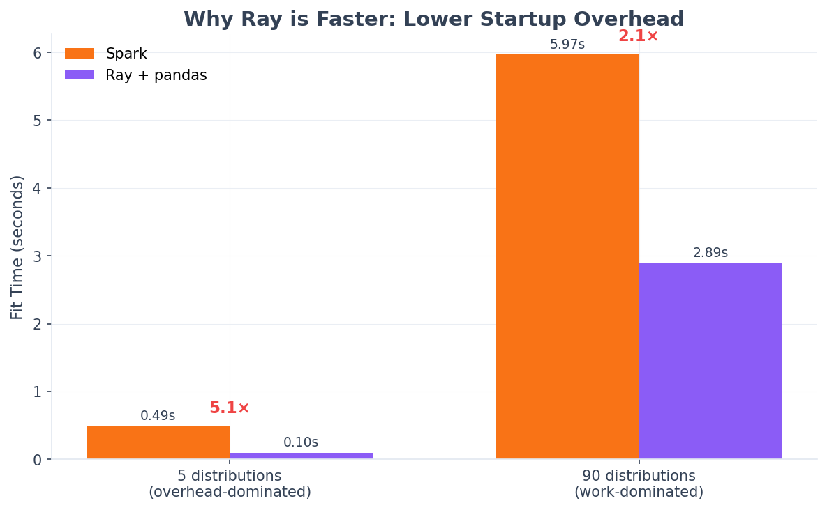
Benchmark Comparison (Auto-generated)

The following benchmarks were run on a local development machine.

Data Size Scaling (90 distributions)

Data Size	Spark	Ray + pandas	Ray Dataset	Fastest
25,000	5.04s	2.89s	4.80s	Ray+pandas
100,000	6.59s	2.98s	4.37s	Ray+pandas
500,000	6.03s	3.20s	4.44s	Ray+pandas
1,000,000	5.16s	2.90s	4.26s	Ray+pandas

Distribution Count Scaling (10K rows)

# Distributions	Spark	Ray + pandas	Ray Dataset	Fastest
5	0.49s	0.10s	1.79s	Ray+pandas
20	0.98s	0.29s	2.04s	Ray+pandas
50	1.53s	0.63s	2.36s	Ray+pandas
90	5.97s	2.89s	4.57s	Ray+pandas
107	6.64s	3.00s	4.36s	Ray+pandas

Running Benchmarks

To run benchmarks locally and generate updated charts:

# Run Spark benchmarks
make benchmark

# Run Ray benchmarks (requires ray installed)
make benchmark-ray

# Generate scaling charts
make benchmark-charts

Benchmark results are saved to .benchmarks/ and charts to docs/_static/.

Copula Sampling Performance (v2.8.0)

The GaussianCopula.sample() method generates correlated multi-column samples efficiently. v2.8.0 introduces two key optimizations:

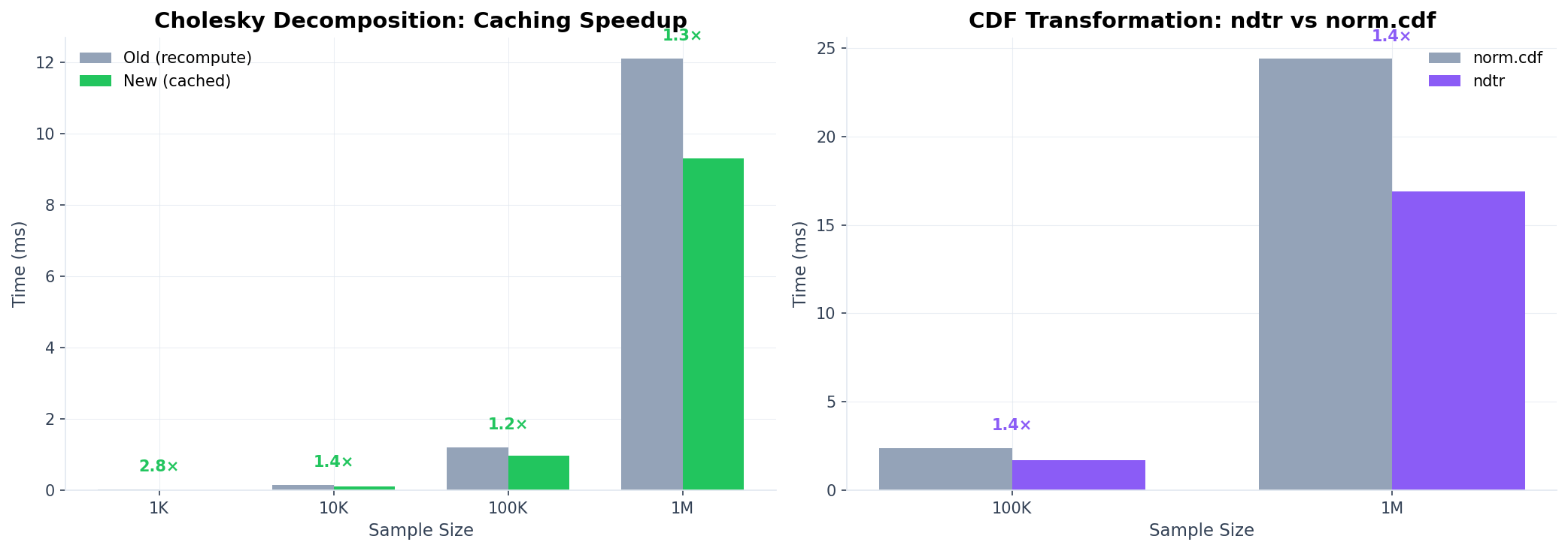
1. Cached Cholesky decomposition: The Cholesky decomposition of the correlation matrix is computed once during copula initialization, not on every sample() call.

2. scipy.special.ndtr: Uses the optimized UFUNC for standard normal CDF instead of scipy.stats.norm.cdf.

These optimizations provide ~1.3-1.5x speedup for the sampling pipeline.

Copula Sampling Benchmarks

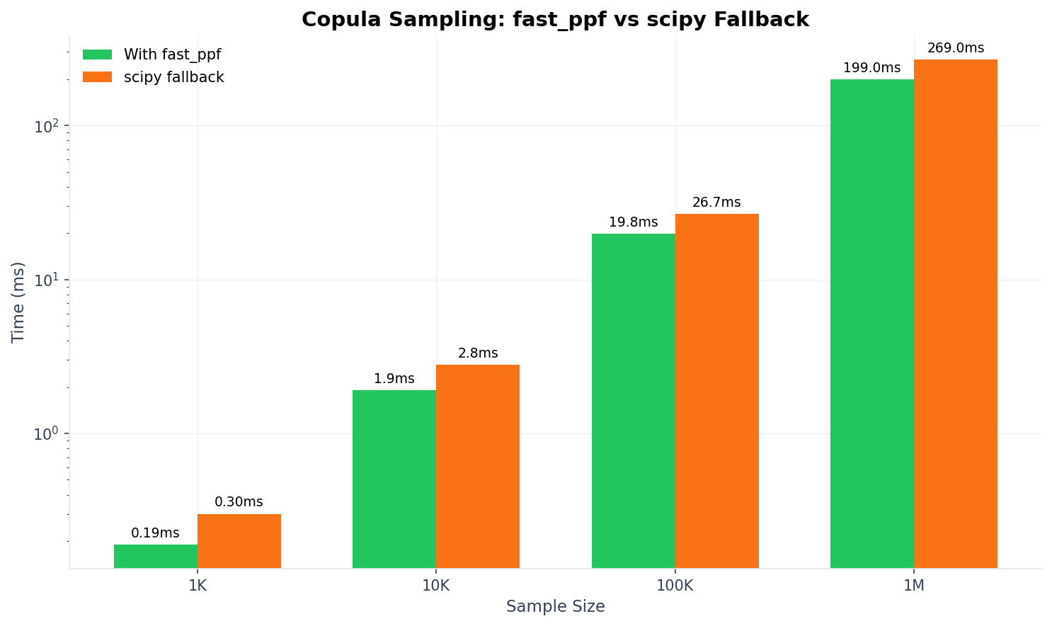
Sample Size	With fast_ppf	scipy fallback	Speedup
1K	0.19 ms	0.30 ms	1.6×
10K	1.9 ms	2.8 ms	1.4×
100K	19.8 ms	26.7 ms	1.4×
1M	199 ms	269 ms	1.4×

v2.8.0 Internal Optimizations

Cholesky Caching (multivariate normal generation):

Sample Size	Old (recompute)	New (cached)	Speedup
1K	0.028 ms	0.010 ms	2.8×
10K	0.15 ms	0.11 ms	1.4×
100K	1.2 ms	0.97 ms	1.3×
1M	12.1 ms	9.3 ms	1.3×

ndtr vs norm.cdf (CDF transformation):

Sample Size	norm.cdf	ndtr	Speedup
100K	2.4 ms	1.7 ms	1.4×
1M	24.4 ms	16.9 ms	1.4×

Best Practices for Copula Sampling

1. Use fast_ppf-supported distributions (norm, gamma, beta, lognorm, weibull_min, uniform, expon) for best performance. These use analytical PPF formulas.

2. Use return_uniform=True for the fastest sampling when you only need correlated uniform samples (skips marginal transformation).

3. For >1M samples, use sample_distributed() with a backend to parallelize across workers.

Related Documentation

• Backend Guide - Detailed backend comparison and configuration

• Lazy Metrics - Lazy metric evaluation for faster workflows

• Pre-filtering - Skip incompatible distributions

• Migrating to v2.0 - Version history and performance improvements